Category Archives: python

Troubleshooting OpenStack the cool way: ini_comparer.py

If OpenStack is already complex enough, troubleshooting OpenStack issues can be a nightmare! If you agree, you might be interested on the ini_comparer script.

The source of most of the issues with OpenStack is usually on the configuration files, which have the “ini” format. This format is not particularly easy to handle by old school “sed” people like me and in addition, the standard configuration files are meant to be self-documented, which means tons of lines of comments and commented options.

Putting this together, we get huge configuration files, with very similar lines and it is a pain in the lower back to check word by word, character by character every single keyword in the file.

So, provided that we have another configuration file that works fine, we can use the ini_comparer python script to do that for us. It can work with a combination of local or remote files. For example, a file on the local machine and another one in a remote one, both files are in the local machine, or both are in remote machines. Continue reading

Logo of BOMSI

The easiest way to install OpenStack: BOMSI GUI

Installing OpenStack is quite difficult, specially for the people who is not really into basically most of IT topics. In my attempt to get started, and after searching for the easiest way to install OpenStack, I ended up writing my own automated tasks in BASH, and at some point I decided to generalice those scripts a little bit more and release them to the community.

I named the installer as BOMSI: the Bash OpenStack Multinode Scripted Installer. Descriptive and catchy, isn’t it? 🙂

BOMSI follows the official install guide at OpenStack Docs for CentOS7, and it does it in plain BASH, so it is easy to understand whatever is going on during the installation, and easily improve it. It’s GPL v2 license, so you are all very welcome to contribute on GitHub repository.

The command line API is very simple and it allows to install OpenStack on a virtual environment with just 3 commans:


git clone https://github.com/julenl/BOMSI.git
cd BOMSI/CentOS7-Kilo/
for NODE in controller compute1 network; do ./bomsi-iso.sh -n=$NODE; done

… and that’s it. In some 15 minutes a horizon dashboard will be waiting for you at http://10.0.0.11/dashboard.

For generating the 3 node virtual environment it is recommended that have 8 or 16 Gb of RAM, a i5 or i7 processor (or equivalent) and some 20 Gb of free space on the hard disk, to host the KVM virtual machines. Ideally the computer should be running Ubuntu, but it should work somehow in other GNU/Linux distributions.

Furthermore, being aware that some people prefer graphical user interfaces (GUIs) to work on the configuration files and execute the options, I also added a very simple GUI.

This GUI can be run the same as the API, but with even less letters on the command line:

git clone https://github.com/julenl/BOMSI.git
cd BOMSI/CentOS7-Kilo/
./bomsi_gui.py

And you’ll get this:
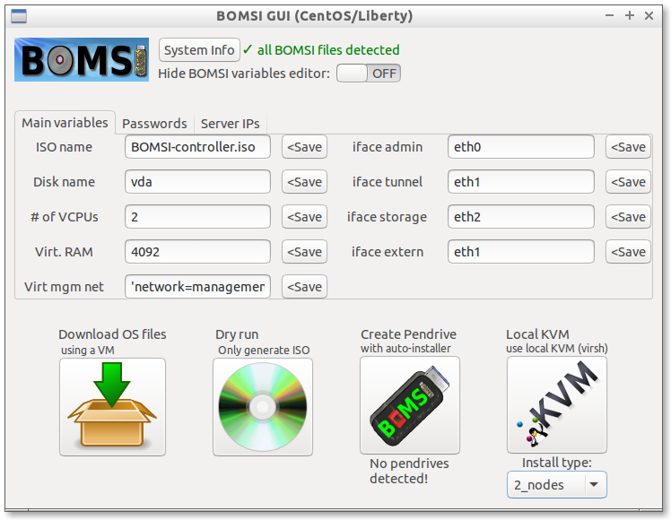
Graphical User Interface for installing OpenStack with BOMSI

If you are OK with the default options, just click on the “Local KVM” square button and wait for some 15 minutes. That’s it.

Additional features of BOMSI:

  • Generate a fully automated multiboot ISO file, which can be burned onto a CD or provisioned via PXE
  • Install this ISO file into a pen-drive
  • Install a temporal CentOS machine with kickstart. This machine can be used to download all necessary packages to allow full offline installations

So… 3 commands, or 3 commands and a click, isn’t this the easiest way to install OpenStack at the moment?

now for HLRN III

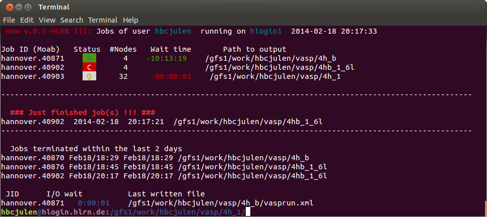
This is a new version of my now python script for monitoring the HLRN III.
I am usually on the Hannover partition, but it should work perfectly in Berlin too.

In this version, I keep all the features of the cluster version except the “gossip” section for checking on who is calculating what and how many resources are they using, since a supercomputer has too many users and we would need a terminal of a couple of square meters.

Screenshot of now HLRN III

now version 0.5 specially modified for working on HLRN III supercomputer in Hannover and Berlin.

Continue reading

cube2xyz: convert cube data to xyz and slize segments/planes

In this post, I introduce my new cube2xyz script for converting cube data into “x,y,z,value” format and optionally creating nice 2D or 3D plots displaying the value of the cube property along a segment or a surface.

.cube files are originally from the Gaussian molecular modeling code, but nowadays can be produced and read by most of the computational chemistry programs. They consist of a lot of blocks of data describing the values of a measured property (charge, spin polarization, electronic density, …) on each point of the space inside the simulation cell.

Continue reading

shrink_traj v0.4: xyz with unit cell info

One of the limitations of xyz coordinate format is generally the lack of extra information, such as the unit cell dimensions or lattice vectors. This can become annoying when we are working with solids, or we want to check whether our molecule has enough space around, in order avoid interaction with its own periodic replicas.
The new shrink_traj v0.4, includes the possibility to include the Jmol readable unit cell info the second line of the xyz file. This way, we can shrink a trajectory (or keep it as it is), and generate a new one which allows us to visualize the unit cell.

It also contains an option to insert Jmol commands directly into the xyz file, such as “background white”, which enables the possibility to customize the view of the structure/trajectory. Continue reading

agr2gpt: convert xmgrace to gnuplot or mathplotlib

Some people seem to think that xmgrace is somehow cool, maybe because it contains an “x” on its name. Y personally prefer gnuplot or mathplotlib, but I got recently some “.agr” files I had to edit, and I finally decided to write a python script called agr2gpt, which makes a simple conversion from xmgrace files to gnuplot script, and extracts the data to different files (one per curve).

This is just the first version, so it just handles basic 2D graphs with several curves.
Besides the x and y data for each curve (unlimited amount of curves), it also parses the “xlabel” the “ylabel” and the legend of each curve.

As in most of my scripts, the “-h” option will provide some extra information about the usage, but in this first version, there are only two options: “-f” for the file name, and “-pl” if you want the pylab window to pop up with the image. Continue reading

now for different supercomputers

I already shared my now script intended for a small “in home” computing cluster. This time, I am sharing two other variations of that script, designed for the queuing systems of two different supercomputers: Mare Nostrum at BSC, Juropa at JSC and HLRN.

Both of them are the predecessors of the newer now script, and they only have the very basic features, but if you need an script that works right out of the box for any of the supercomputers mentioned above, this is the quick solution.

Continue reading

pw2cellvec: monitor vc-relax convergence in QE

When running a cell relaxation, it is sometimes nice to monitor what is going on with the cell parameters. If you run the cell relaxation with Quantum Espresso, you can use my python script “pw2cellvec” to parse all the information you need.

So, first of all, run a “vc-relax” calcuculation with a large (about 2 times bigger) cutoff for both wavefunction (ecutwfc) and charge (ecutrho) and wait for a couple of iterations. These calculations are very expensive, due to the large cutoffs.

Then, just run the script and you will get something like this:

user> pw2cellvec.py -o pwout
- -
AA a= 6.02104498011 b= 6.02109150665 c= 9.45688483193 Vol.= 296.919819153
au a= 11.3781260524 b= 11.3782139748 c= 17.8709224124 c/a= 1.57063846279
alpha= 89.9989981833 beta= 90.0012313781 gamma= 119.99694776
- - Continue reading

pw2gap: Quick Homo/Lumo gap check for QE

In order to check the Homo/Lumo gap from a Quantum Espresso (pw.x) calculation it is possible to plot the Density Of States and estimate the distance of empty states around the Fermi level (E=0), but what about if we only want a numerical (accurate) value?
This can be done very quick with “pw2gap” script, which can be downloaded from here.

It goes trough all the eigenvalues at the end of the output, including the case of spin-polarization (spin up/down) and k-points, and it simply prints the energies of the HOMO and LUMO orbitals as well as, of course, the difference between them. As simple as that.

It looks like this (for the example of the wustite):

user> pw2gap.py -o pwout
HOMO= 9.4503 LUMO= 11.5898 eV
H/L GAP = 2.1395

sum_states.py: Nice DOS plots from QE outputs

Once, I was making some DOS figures with quantum espresso by using the sumpdos.x program by Andrea Ferretti (included in the QE package), but I felt that I am missing some features. Thereby, I wrote my own script, which does something similar, but it is much more automatized, it is faster to use, and it even produces ready-to-publish graphs automatically.

It is part of the quantum espresso distribution, so if you have the source code of quantum espresso, you have it in the …/*espresso*/PP/tools/sum_states.py. If you don’t have it, or you just want to read the source-code online, you can check for sum_states.py in the quantum espresso repository. Continue reading